Problem solving
Worked exercise 1
Let w is a word over the alphabet  . This string can be considered as a binary representation of a natural number. Denote this number by
  and let
 .
.
Construct automaton M which recognizes this language.
Hint

 .
.
How do these equality change if we calculate modulo 3?
Solution
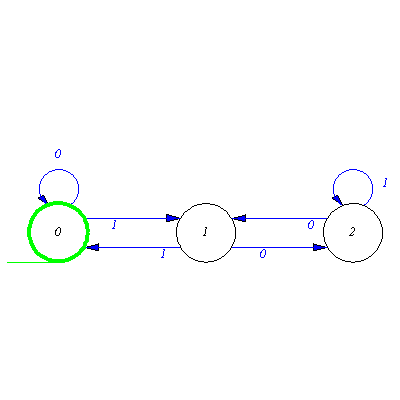
Let the states of automaton be the complete residue system  modulo 3. Let
  be the alphabet of automaton. For all state
  and
and  let us define
 .
.
Some example for transitions:


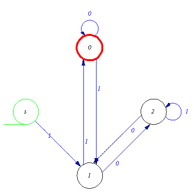
Now we can generate the automaton and display the transition graph. Plotaut gives nicer picture when using option line.
| > |
M:=genaut([0,0,0,0,1,1,1,0,2,1,1,0,2,0,1,2,1,2],0,0); |
![[{0, 1, 2}, {`0`, `1`}, delta, {0}, {0}]](images/Automata constructions_76.gif) |
(2.1.1) |
Check some input words for recognition.
| > |
accept(M,w,tr1,sho); # EoP |
-Delta begins with 0
-Delta(0,`1`) = 1
-Delta(1,`0`) = 2
-Delta(2,`0`) = 1
-Delta(1,`1`) = 0
-Delta(0,`0`) = 0 |
 |
| Result of Delta: |
 |
 |
| Result of accept: |
 |
(2.1.3) |
Display the words of length 0..5 belonging to L(M).
| > |
langaut(M,0..5,group,show); |
| length 0: |
 |
| length 1: |
 |
| length 2: |
 |
| length 3: |
 |
| length 4: |
 |
| length 5: |
 |
| Result of langaut: |

 |
(2.1.4) |
The result is much more comprehensible if we convert the binary string to decimal numbers.
| > |
map(x->convert(x,decimal,2),%); |
 |
(2.1.5) |
The result is self explanatory.
On the same time notice, that leading zeros are present in binary strings (see worked exercise 2).
Worked exercise 2
Alter the automaton M constructed in the former exercise so that it does not recognize binary strings with leading zeros.
Solution
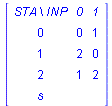
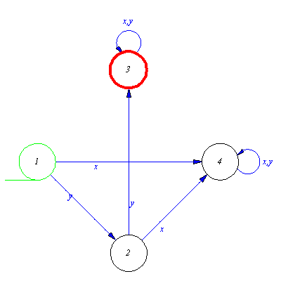
Display the transition table of M.
We have to introduce a new initial state for which the input signal 1 is defined only. Denote the new start state by s and add it to the automaton.
![[{0, 1, 2, s}, {`0`, `1`}, xT, {0, s}, {0}]](images/Automata constructions_98.gif) |
(2.2.2) |
Now we have two initial states. The old one has to be erased.
![[{0, 1, 2, s}, {`0`, `1`}, xT, {s}, {0}]](images/Automata constructions_99.gif) |
(2.2.3) |
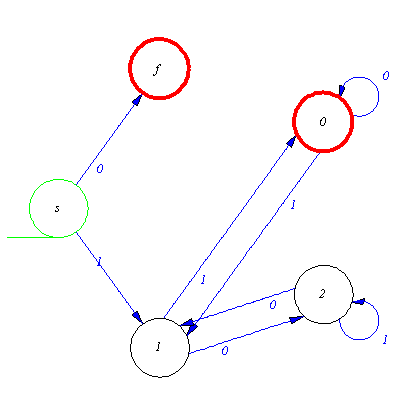
For the moment there is no transition defined for the new initial state. The question is to which state have to move the automaton from state s when reading the input signal 1? The answer is that the result of new transition has to be the same as in the original case, i.e.
 .
.
| > |
N:=addaut(N,tra=[s,1,1]);plotaut(N); |
Check the result...
| length 0: |
|
| length 1: |
|
| length 2: |
 |
| length 3: |
 |
| length 4: |
 |
| length 5: |
 |
 |
(2.2.5) |
| > |
map(x->convert(x,decimal,2),%); |
 |
(2.2.6) |
Almost correct. Unfortunately we lost the string `0`. In order to accept it we add a new final state to which the automaton moves when reading `0`.
| > |
N:=addaut(N,tra=[s,0,f],fin=f); plotaut(%); |
| > |
map(x->convert(x,decimal,2),langaut(N,0..6)); |
 |
(2.2.7) |
Worked exercise 3
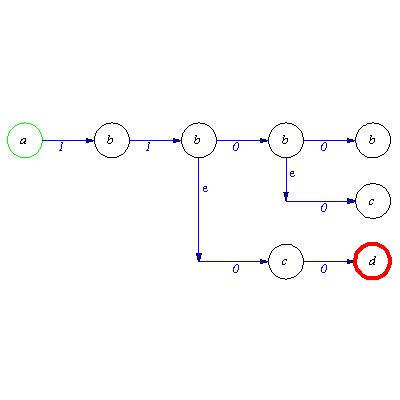
Construct automaton which recognizes a word w over the alphabet  if and only if the first signal of w is 1 and w ends by two zeros. Check the type of automaton. Determine and visualize the possible set of runs associated with different input words.
Solution
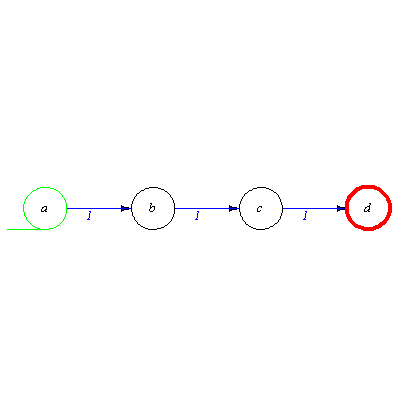
Following György Pólya let us begin by solving a simpler problem. Construct automaton which recognizes the one element set  . The solution is evident.
| > |
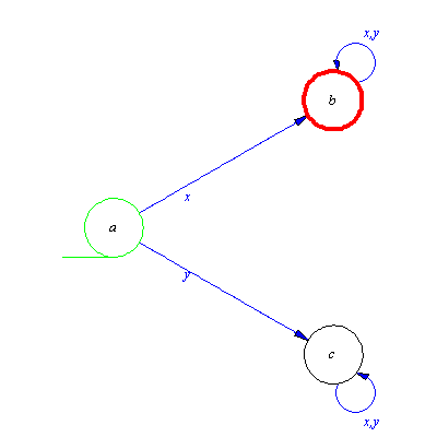
M:=genaut([a,1,b],a,b);plotaut(%); |
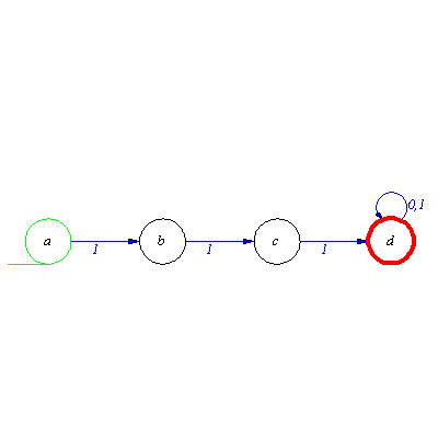
How should we alter this automaton to recognize words of the form 1q, where q is arbitrary word over the alphabet  This requirement prescribes that the automaton should be able to continue the calculation after the first 1, whatever is the suffix of the input word. This can be reached by adding two new transitions, namely two loops. Both of the input signal should leave the state b unchanged.
| > |
M:=addaut(M,transition={[b,0,b],[b,1,b]});plotaut(%); |
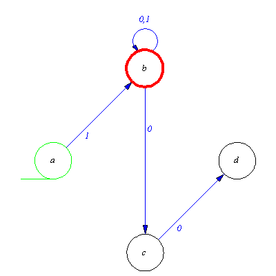
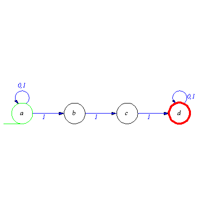
In the and we have to alter the automaton so that it ends its operation with two zeros. This requires two new states. From state b the input signal 0 should move M to a new state, and a second 0 from this state to another state.
| > |
M:=addaut(M,transition={[b,0,c],[c,0,d]});plotaut(%); |
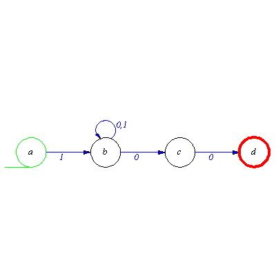
The transitions seem to be correct. The recognition can begin with 1, continue with arbitrary word in the state b, and end by two zeros. But from now on the state b is not a correct final state, the correct recognition is made by the state d. So we have to erase b from the set of final state and add state d to it.
| > |
M:=addaut(delaut(M,final=b),final=d); plotaut(%); |
The option line may result in more nicer picture.
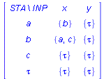
The datastructure of M can be checked by the type procedure. We see that automaton M is neither deterministic nor complete.
 |
(2.3.1) |
 |
(2.3.2) |
 |
(2.3.3) |
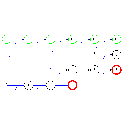
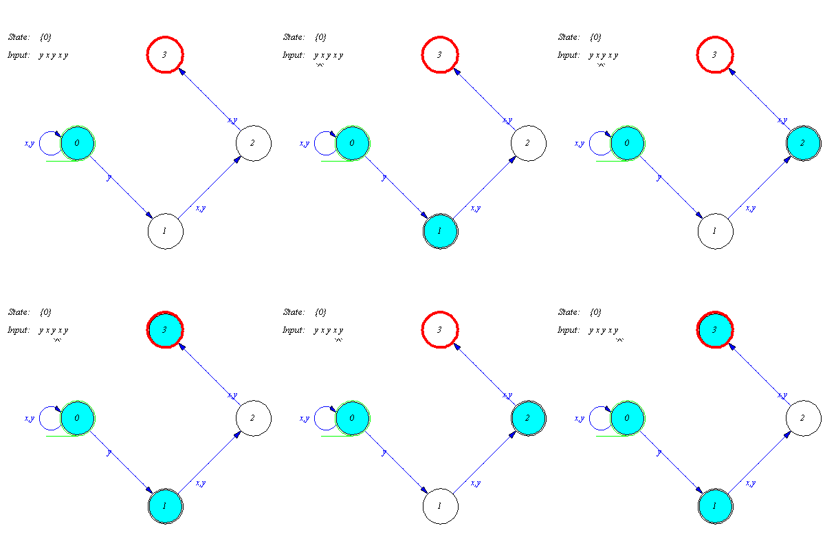
The sequence of SoPS (set of of possible state) and the set of possible runs can be produced by using Delta.
 |
(2.3.4) |
-Delta begins with {a}
-Delta({a},`1`) = {b}
-Delta({b},`1`) = {b}
-Delta({b},`0`) = {b, c}
-Delta({b, c},`0`) = {b, c, d} |
 |
(2.3.5) |
![{[a, b, b, b, b], [a, b, b, b, c], [a, b, b, c, d]}](images/Automata constructions_132.gif) |
(2.3.6) |
Worked exercise 4
Create deterministic and complete automaton which recognizes the language { |
|  }.
}.
As before begin with a much simpler problem. Erase the letter y at the end of words to be accepted and consider first the language
{ |
|  }.
}.
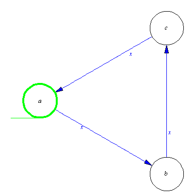
This language consists of words like  , xxx, xxxxxx, xxxxxxxxx, ...etc, which can be easily recognized by a three state automaton.
| > |
M:=genaut([a,x,b,b,x,c,c,x,a],a,a); |
![[{a, b, c}, {x}, delta, {a}, {a}]](images/Automata constructions_139.gif) |
(2.4.1) |
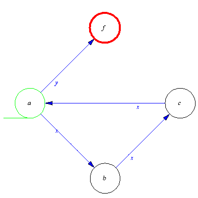
Now we alter this automaton so that it recognize words y, xxxy, xxxxxxy, xxxxxxxxxy, ...etc. We have nothing else to do than to create a new transition for state a and the input signal y. The result of this transition must be the new final state, which on the same time can be none of the existing states (why?). So we have to establish a new state, say f. As the state a is no more final state, we first delete it from set of final states and then add a new transition and a new final state.
| > |
N:=addaut(delaut(M,fin=a),tra=[a,y,f],final=f); |
![[{a, b, c, f}, {x, y}, xT, {a}, {f}]](images/Automata constructions_141.gif) |
(2.4.2) |
 |
(2.4.3) |
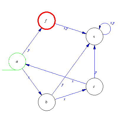
This automaton is the solution of our exercise. Let us consider the characteristic features of this automaton. It is deterministic, but not complete. Indeed, several transitions are not defined. These transitions, however, are irrelevant from the point of view of word recognition. The equivalent complete automaton can be created by procedure ConCom (CONstruct Complete automaton).
![[{a, b, c, f, tau}, {x, y}, delta, {a}, {f}]](images/Automata constructions_144.gif) |
(2.4.4) |
Worked exercise 5
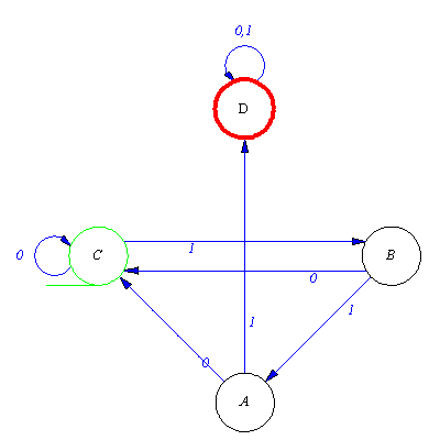
Create deterministic automaton which recognizes a word over the alphabet {0,1} if and only if it contains three consecutive 1s .
Similar to the solution of previous exercise we divide the problem into simpler subproblems. The recognition of three consecutive 1s is an easy task.
| > |
M:=genaut([a,1,b,b,1,c,c,1,d],a,d); |
![[{a, b, c, d}, {`1`}, delta, {a}, {d}]](images/Automata constructions_146.gif) |
(2.5.1) |
The words we have to recognize contains a subword 111, and besides it can have an arbitrary suffix ...
| > |
M:=addaut(M,transition={[d,0,d],[d,1,d]}); |
![[{a, b, c, d}, {`0`, `1`}, xT, {a}, {d}]](images/Automata constructions_148.gif) |
(2.5.2) |
... and an arbitrary prefix.
| > |
M:=addaut(M,transition={[a,0,a],[a,1,a]}); |
![[{a, b, c, d}, {`0`, `1`}, xT, {a}, {d}]](images/Automata constructions_150.gif) |
(2.5.3) |
 |
(2.5.4) |
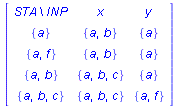
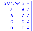
This automaton is neither complete nor deterministic. If we insisted on obtaining a deterministic automaton we use procedure ConDet (CONstrunct DETereministic automaton). As the stets of resulted deterministic automaton are states fro the sake of simplicity it worth to rename them.
![[{{a}, {a, b}, {a, d}, {a, b, c}, {a, b, d}, {a, b, c, d}}, {`0`, `1`}, delta, {{a}}, {{a, d}, {a, b, d}, {a, b, c, d}}]](images/Automata constructions_153.gif)
![[{{a}, {a, b}, {a, d}, {a, b, c}, {a, b, d}, {a, b, c, d}}, {`0`, `1`}, delta, {{a}}, {{a, d}, {a, b, d}, {a, b, c, d}}]](images/Automata constructions_154.gif) |
(2.5.5) |
![[{A, B, C, D, E, F}, {`0`, `1`}, delta, {A}, {B, D, F}]](images/Automata constructions_155.gif) |
(2.5.6) |
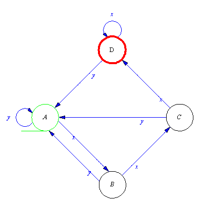
To produce the minimal state automaton recognizes the same language we use the procedure ConMin (CONstrunct MINimal automaton).
| > |
plotaut(renaut(ConMin(N),sta=A)); |
More exercises
Construct automata recognizing the following languages:
a) 
b) 
c) 
d) 
e) 
f) 
g) 
h) Describe L(M) for the following automaton:
| > |
M:=genaut([1,a,2,1,b,3,2,a,3,2,b,1,3,a,1,3,b,2],1,{1}); |
![[{1, 2, 3}, {a, b}, delta, {1}, {1}]](images/Automata constructions_165.gif) |
(2.6.1) |
Automata constructions
We find tools in aut package for different construction widely used in the course of investigating finite automata. The subset construction for establishing equivalent deterministic automata, union and product constructions for recognizing union and intersection of acceptable languages and last but not lest the factor construction to reduce the number of states of deterministic automata without changing the language recognizing power.
Union construction
We are looking for an automaton which recognizes a word w over the alphabet  if and only if w does not contain two different signal and a length of all words is congruent 0 modulo 3. This language equals to the union of two very simple languages:
 .
.
It is easy to construct automata recognizing these languages.
| > |
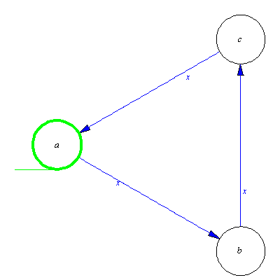
M:=genaut([a,x,b,b,x,c,c,x,a],a,a): printaut(M); |
| > |
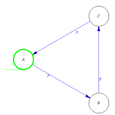
N:=genaut([A,y,B,B,y,C,C,y,A],A,A):printaut(N); |
As the union construction insists on automata with the same alphabet, we have to supplement the alphabet of both automaton.
| > |
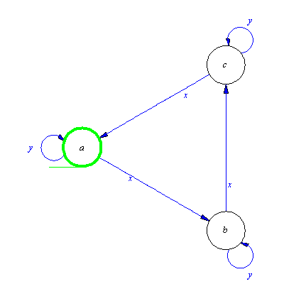
M:=addaut(M,inp=y):printaut(M); |
| > |
N:=addaut(N,inp=x):printaut(N); |
The union construction can be performed by procedure Construct, whose first parameter is the name of construction, while the second the list of automata on which the construction is to be performed.
| > |
P:=Construct(`union`,[M,N]); |
![[{A, B, C, a, b, c}, {x, y}, delta, {A, a}, {A, a}]](images/Automata constructions_180.gif) |
(3.1.5) |
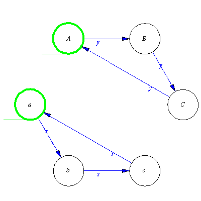
Display the transition graphs of these three automata to see what have we done.
|
|
| > |
plotaut(P,
sort=[a,b,c,C,B,A]); |
|
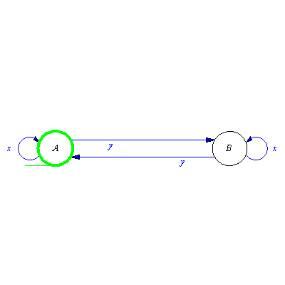
The transition graph of P is the union of the transition graphs of M and N. Construct simply joined the graphs of two automata by simply putting them next to each other. Automaton P recognizes the union of L(M) and L(N), indeed. If it gets an input word, it makes a choice. It decides with which initial state it begins to work, and works according to that automaton whose start state it has been chosen.
Product construction
Let us start with generating two automata M and N, and construct a third one which recognizes the intersection of the languages L(M) and L(N).
| > |
M:=genaut([a,x,b,b,x,c,c,x,a,a,y,a,b,y,b,c,y,c],a,a):plotaut(%); |
This automaton is very similar to that we introduced in the previous section. It can be seen that this three state automaton recognizes a word w over the alphabet  if and only if the number of occurrences of x in w can be divided by 3. Let the next automaton be one which recognizes words having even number of y.
| > |
N:=genaut([A,y,B,B,y,A,A,x,A,B,x,B],A,A):plotaut(%); |
Again we use the procedure Construct, but now the name of construction is product instead of union.
| > |
P:=Construct(product,[M,N]); |
![[{[a, A], [a, B], [b, A], [b, B], [c, A], [c, B]}, {x, y}, delta, {[a, A]}, {[a, A]}]](images/Automata constructions_187.gif) |
(3.2.1) |
What kind of automaton we have obtained? One thing is clear: the states of new automaton in ordered pairs. The first component of all pairs is a state of automaton M, while the second comes from N. The initial state is created from the initial states of M and N, and the same is true for final state. A closer look at the transition tables clarify the operation of new automaton.
Observe that the automaton P synchronizes the operation of automata M and N in such a way that P works on the first component of is states according to the transition function of M and on the second component of the states works according to automaton N, i.e.
![delta(P, s, xi) = [delta(M, s[1], xi), delta(N, s[2], xi)]](images/Automata constructions_197.gif)
holds for every state s and input signal ξ. Consider the transition graph of P.
Although we feel that there must be some symmetry in this graph, it not really nice. We can, however produce another graph which clearly shows the beautiful inner structure of automaton P.
| > |
par:=[a,A]=[-1,0],[b,A]=[0,0.5],[c,A]=[1,0]:
par:=par,[a,B]=[-1,1],[b,B]=[0,1.5],[c,B]=[1,1]:
plotaut(P,par); |
Instead of trying to prove the equality

we may ask how has automaton P constructed? Call procedure Construct by using the options state and show.
| > |
Construct(product,[M,N],state,show); |
![`SoGS in step 0 =`, {[a, A]}](images/Automata constructions_201.gif) |
![`SoGS in step 1 =`, {[a, A], [a, B], [b, A]}](images/Automata constructions_202.gif) |
![`SoGS in step 2 =`, {[a, A], [a, B], [b, A], [b, B]}](images/Automata constructions_203.gif) |
![`SoGS in step 3 =`, {[a, A], [a, B], [b, A], [b, B], [c, B]}](images/Automata constructions_204.gif) |
![`SoGS in step 4 =`, {[a, A], [a, B], [b, A], [b, B], [c, A], [c, B]}](images/Automata constructions_205.gif) |
![`SoGS in step 5 =`, {[a, A], [a, B], [b, A], [b, B], [c, A], [c, B]}](images/Automata constructions_206.gif) |
![`SoGS in step 6 =`, {[a, A], [a, B], [b, A], [b, B], [c, A], [c, B]}](images/Automata constructions_207.gif) |
| Result of Compose: |
![[{[a, A], [a, B], [b, A], [b, B], [c, A], [c, B]}, {x, y}, delta, {[a, A]}, {[a, A]}]](images/Automata constructions_208.gif) |
(3.2.5) |
We see that Construct performed steps namely six steps. In each step it created an SoGS which stands for Set of Generated States. These generated set form an increase sequence. The last SoGS is the set of state of the generated automaton. At this stage it's enough, further details are coming later.
Subset construction
As usual we begin with generating a nondeteministic automaton  and immediately plot its transition graph.
| > |
M:=genaut([a,{x,y},a,a,x,b,b,x,c,c,y,f]); |
![[{a, b, c, f}, {x, y}, delta, {a}, {f}]](images/Automata constructions_210.gif) |
(3.3.1) |
Subset construction aims to construct equivalent deterministic automaton, i.e. a deterministic automaton P which recognizes the same language. Again we use Construct but now the name of construction is set. The second parameter is a one element list.
![[{{a}, {a, b}, {a, f}, {a, b, c}}, {x, y}, delta, {{a}}, {{a, f}}]](images/Automata constructions_212.gif) |
(3.3.2) |
First of all we check, if the result is dereteministic.
 |
(3.3.3) |
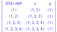
Now let's take a look on the states of new automaton. Remember that in case of product construction Construct established ordered pairs. Now we have got sets.More precisely all these sets are subset of the set of states of the original automaton. What about the transition function of P?
It is easy to check, that

for all state A and input signal ξ. Ask Construct to tell something about its operation. As before use options show, and state.
| > |
Construct(set,[M],show,state); |
 |
 |
 |
 |
 |
| Result of Compose: |
![[{{a}, {a, b}, {a, f}, {a, b, c}}, {x, y}, delta, {{a}}, {{a, f}}]](images/Automata constructions_226.gif) |
(3.3.6) |
In this case Construct also generated an increasing sequence of sets and the last generable set became the set of states of new automaton. Now we are eager to now more about what happens behind the scenes. We ask further details by using option trace2.
| > |
Construct(set,[M],show,state,trace2); |
 |
[{a}]->pop({a})->[]
.delta({a},x) = {{a, b}}
..push({a, b}): [{a, b}]
.delta({a},y) = {{a}} |
 |
[{a, b}]->pop({a, b})->[]
.delta({a, b},x) = {{a, b, c}}
..push({a, b, c}): [{a, b, c}]
.delta({a, b},y) = {{a}} |
 |
[{a, b, c}]->pop({a, b, c})->[]
.delta({a, b, c},x) = {{a, b, c}}
.delta({a, b, c},y) = {{a, f}}
..push({a, f}): [{a, f}] |
 |
[{a, f}]->pop({a, f})->[]
.delta({a, f},x) = {{a, b}}
.delta({a, f},y) = {{a}} |
 |
| Result of Compose: |
![[{{a}, {a, b}, {a, f}, {a, b, c}}, {x, y}, delta, {{a}}, {{a, f}}]](images/Automata constructions_232.gif) |
(3.3.7) |
We have got the answer we wanted. We see 'push' and 'pop' which tells us evidently that Construct uses a stack. At the very beginning SoGS consists of the one element and the stack contains . Next it takes the element s from the top of stack (pop it), and calculate
  and if this set in not belongs to SoGS then it is supplemented to it. The same is done for the input signal y, i.e. if
  then
then  . This ends step 1, and all this is repeated until the stack is not empty. The last SoGS is the set of states of generated automaton.
Summary
The main concept behind the procedure Construct can be summarized as follows.
1. Imagine a set , a universe from which we will choose the states of new automaton.
2. Choose one element of universe, this will be the initial state of new automaton.
3. Specify how the new transition function works on the elements of universe.
4. Perform the algorithm described earlier, i.e. beginning with the initial state calculate the sequence of SoGSs. The last SoGS serves as the set of state of new automaton.
5. Specify the final state(s) of new automaton.
6. Put all these element to a list and build the new automaton.
The Construct procedure
We demonstrate these process with the product construction. First of all we need two automaton.
| > |
M:=genaut([a,x,b,b,{x,y},b,a,y,c,c,{x,y},c],a,{b});plotaut(%); |
| > |
N:=genaut([1,y,2,2,y,3,3,{x,y},3,1,x,4,2,x,4,4,{x,y},4],1,{3});plotaut(%); |
Now we do not care of what languages are accepted by these automata. We focus on construction instead. The first step of implementation is to declare that the set input signal of new automaton is the same as that of M. Recall the second component of an automaton type object is nothing else that the alphabet.
 |
(3.4.1) |
Next we specify the initial state of new automaton. Our universe is the Cartesian product of the set of states of two automaton. The ordered pair consisting of the initial states of two automata is declared as the initial state of new automaton.
| > |
newini:=Cartesian(M[4],N[4]); |
![{[a, 1]}](images/Automata constructions_242.gif) |
(3.4.2) |
The most important step is to specify the rules, which determines the operation of new automaton. This is implemented by the procedure newtra. This procedure supposes to get a list of automata, a state and an input signal.
| > |
newtra:=(l,a,x)->{[Delta(l[1],a[1],x),Delta(l[2],a[2],x)]}; |
![proc (l, a, x) options operator, arrow; {[Delta(l[1], a[1], x), Delta(l[2], a[2], x)]} end proc](images/Automata constructions_243.gif) |
(3.4.3) |
In the end the final states are stored in the variable newfin.
| > |
newfin:=Cartesian(M[1],N[5]) union Cartesian(M[5],N[1]); |
![{[a, 3], [b, 1], [b, 2], [b, 3], [b, 4], [c, 3]}](images/Automata constructions_244.gif) |
(3.4.4) |
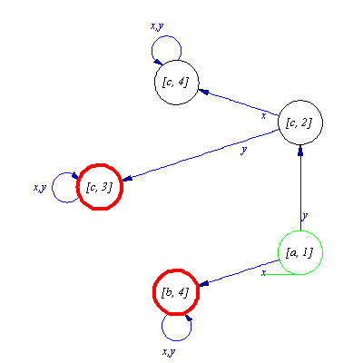
The last step of the implementation is to call procedure Compose which is the "construction engine" of aut package. Actually it is Compose which performs the algorithm we described before.
| > |
Compose(generate,[M,N],[newinp,newtra,newini,newfin]);
|
![[{[a, 1], [b, 4], [c, 2], [c, 3], [c, 4]}, {x, y}, delta, {[a, 1]}, {[b, 4], [c, 3]}]](images/Automata constructions_245.gif) |
(3.4.5) |
| > |
plotaut(%,sort=[[c,3],[b,4]]); |
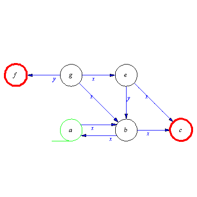
To demonstrate the power if Compose we give two further useful application. Consider a new automaton M .
| > |
M:=genaut([a,x,b,b,x,{c,a},e,x,c,e,y,b,g,x,{e,b},g,y,f],a,{f,c}); |
![[{a, b, c, e, f, g}, {x, y}, delta, {a}, {c, f}]](images/Automata constructions_247.gif) |
(3.4.6) |
| > |
plotaut(M,a=[-1,0],b=[0,0],c=[1,0],g=[-1,1],e=[0,1],f=[-2,1],plotpar=[scaling=constrained]); |
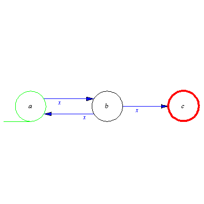
It is easy to see that states  a redundant states. Neither of them can take part in word recognition. To show another useful application of Compose we construct the initially connected subautomaton of M, i.e. we get rid of the unnecessary states.
| > |
newinp:=M[2];
newini:=M[4];
newtra:=(l,a,x)->Delta(l[1],a,x);
newfin:=M[5]; |
| > |
N:=Compose(generate,[M],[M[2],newtra,newini,newfin]); |
![[{a, b, c}, {x, y}, delta, {a}, {c}]](images/Automata constructions_254.gif) |
(3.4.8) |
Although N has got two input signals x and y it haven't got any y-transition. So N is not of type complete. Construct a new automaton N from M by adding a new state τ to the set of states of M. Next keep all defined transition of M unchanged in N and specify every undefined transition of M as τ in N.
| > |
newtra:=proc(l,a,x)
if a=tau then {tau}
elif Delta(l[1],a,x,set)={} then
{tau}
else
Delta(l[1],a,x,set)
fi
end; |
| > |
newinp:=N[2];
newini:=N[4];
newfin:=N[5]; |
| > |
N:=Compose(generate,[N],[newinp,newtra,newini,newfin]); |
![[{a, b, c, tau}, {x, y}, delta, {a}, {c}]](images/Automata constructions_268.gif) |
(3.4.11) |
| > |
plotaut(N,tau=[1,1],c=[2,0],line);
|
References
[1] A.V. Aho, J.E. Hopcroft & J.D. Ullman: Data structures and algorithms. - Addison-Wesley, Reading, Mass. 1983
[2] K.J.Fuchs, Computer Algebra Systems in Mathematic Education, International Symposium - Anniversary of Pollack Mihály College of Engineering, 2002
[3] F. Gécseg & I. Peák: Algebraic theory of automata. - Akadémiai Kiadó, Budapest 1972.
[4] J. E. HOPCROFT AND J. D. ULLMAN, Introduction to Automata Theory, Languages, and Computation, Addison- Wesley, Reading, MA, 1979.
[5] Kozen: Automata and Computability. - Springer-Verlag, New York, 1997.
[6] W. Lindler, CAS-Supported Multiple Representations in the Elementary Linear Algebra, The case of Gaussian Algorithm, International Symposium - Anniversary of Pollack Mihály College of Engineering, 2002
[7] M.B. Monagan, K.O Geddes, K.M. Heal, G.Labahm, S.M.Vorkoetter, J. McCaron. P.DeMarco: Maple 13 Introductory Programming Guide -Waterloo Maple , 2002
[8] M.B. Monagan, K.O Geddes, K.M. Heal, G.Labahm, S.M.Vorkoetter, J. McCaron. P.DeMarco: Maple 13 Advanced Programming Guide -Waterloo Maple , 2002
[9] O. Wurnig, From th first use of the computer up to the integratin of DERIVE in the teaching of mathematics, IGJ Vol 3, No.1. p.11-24, 1996
![]() is a final state then we say the automata accepts or recognizes the word
is a final state then we say the automata accepts or recognizes the word ![]() .
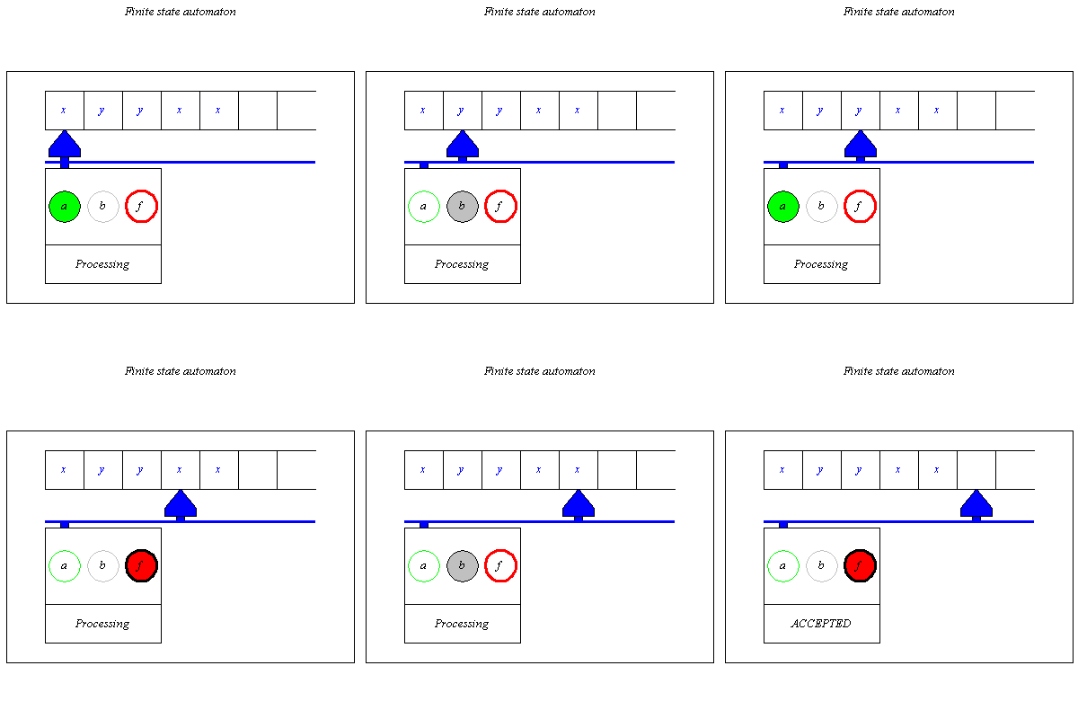
. 
![]() .
. ![]() . This function determines the next state to which the automaton moves from the current state in response to reading current input signal. As we see
. This function determines the next state to which the automaton moves from the current state in response to reading current input signal. As we see ![]() works on pairs of the form
works on pairs of the form ![]() where
where ![]() is a state and
is a state and ![]() is an input signal. The value
is an input signal. The value ![]() is the next state.
is the next state. ![]() prescribe that the input signal x moves the automaton from state 1 to state 2. Note, furthermore, that we use Maple's table datastructure to implement the transition function. In the sequel we do not distinguish the transition function from its implementation.
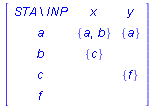
prescribe that the input signal x moves the automaton from state 1 to state 2. Note, furthermore, that we use Maple's table datastructure to implement the transition function. In the sequel we do not distinguish the transition function from its implementation. ![]() tells nothing about the behavior of transition function except its name. What we need is a better representation. The procedure printaut is used to display the transition table of automata.
tells nothing about the behavior of transition function except its name. What we need is a better representation. The procedure printaut is used to display the transition table of automata. 
![]() and the column labeled by the input signal
and the column labeled by the input signal ![]() contains
contains ![]() . It is very important to see, that our notion of automaton is nondeterministic. Indeed the next state is not uniquely determined by the current state and input signal. For example
. It is very important to see, that our notion of automaton is nondeterministic. Indeed the next state is not uniquely determined by the current state and input signal. For example ![]()
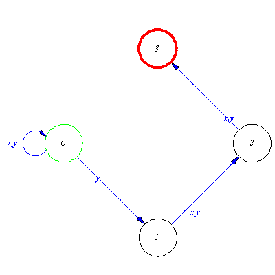
![]() and every input signal
and every input signal ![]() there exists at most one arrow which is labeled by
there exists at most one arrow which is labeled by ![]() and whose starting point is
and whose starting point is ![]() then the automaton is deterministic. Completeness of the transition function provides at least one arrow for every state and input signal.
then the automaton is deterministic. Completeness of the transition function provides at least one arrow for every state and input signal. 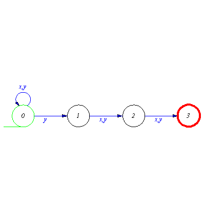
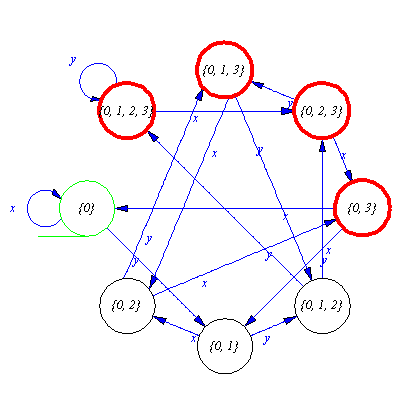
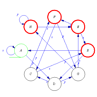
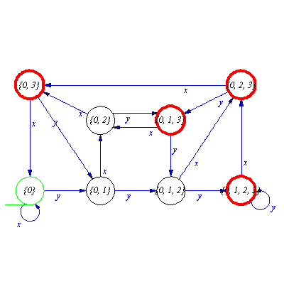

![]() which can be interpreted that the nondeterministic automaton M moves from the start state either to the state 0 or to the state 3 after reading the input word w.
which can be interpreted that the nondeterministic automaton M moves from the start state either to the state 0 or to the state 3 after reading the input word w. 